
Voxel Vision using Maxillofacial CBCT: Clinical Applications of the Maximum Intensity ProjectionDr. William C. Scarfe BDS, FRACDS, MS
Associate Professor Dr. Allan G. Farman BDS, PhD, MBA, DSc Professor Dept. of Surgical/Hospital Dentistry University of Louisville School of Dentistry Louisville, Kentucky, 40292, USA From the Summer 2007 AADMRT Newsletter
The volumetric data set comprises a 3D block of cubes, known as voxels, each representing a specific degree of x-ray absorption. The dimensions of each voxel determines the 3D resolution of the image. CBCT units provide voxel resolutions that are isotropic--equal in all 3 dimensions. This produces submillimeter resolution, currently ranging from 0.4 mm to as low as 0.0936 mm.
Voxel Vision: Image Display Modes The availability of CBCT technology provides the dental clinician with increasing choice of image display formats. The volumetric dataset is a compilation of all available voxels and, for most CBCT devices, is presented to the clinician on screen as secondary reconstructed images in three orthogonal planes (axial, sagittal and coronal) (Figure 1). |


|


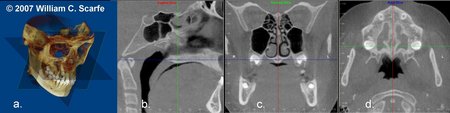
Figure 1. Standard display modes of CBCT volumetric data. a) Volumetric 3D representation of hard tissue showing the three orthogonal planes in relation to the reconstructed volumetric dataset. Green is coronal, Red is sagittal and Blue is axial. Each orthogonal plane has multiple thin slice sections in each plane b) representative sagittal image, c) representative coronal image and d) representative image. (Images produced using Dolphin 3D, Chatsworth, CA)
Because of the isotropic nature of the volumetric dataset, clinicians are now able to evaluate data sets by slicing them non-orthogonally. Although various CBCT systems have unique capabilities and functionality, most provide options for various non-axial 2D images referred to as multi-planar reformation (MPR). Such MPR modes include oblique, curved planar reformation, and serial trans-planar reformation. (Figure 2)
Because of the isotropic nature of the volumetric dataset, clinicians are now able to evaluate data sets by slicing them non-orthogonally. Although various CBCT systems have unique capabilities and functionality, most provide options for various non-axial 2D images referred to as multi-planar reformation (MPR). Such MPR modes include oblique, curved planar reformation, and serial trans-planar reformation. (Figure 2)
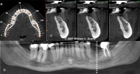
Figure 2. Multiplanar reformatted (MPR) images. A curved planar MPR is accomplished by aligning the long axis of the imaging plane with a specific anatomic structure, most commonly the dental arch (a.), pro- viding familiar panorama-like thin-slice images (b). In addition serial trans-planar images are often generated providing a series of thin (e.g., 1 mm) stacked sequential images orthogonal to the curved planar reforma- tion (b. dashed white lines). Resultant cross-sectional images (c.) are useful in the assessment of specific morphologic features such as alveolar bone height and width as well as the location of the inferior alveolar canal for implant site assessment. (Images generated using i-CAT CBCT; Danaher/Imaging Sciences International, Hatfield, PA)
Because of the large number of component slices in any MPR image and the difficulty in relating adjacent structures, a number of methods have been developed to visualize adjacent voxels -- providing for Voxel Vision. There are essentially two techniques that can be applied to volumetric CBCT data to accomplish this.
1) Ray Sum or Ray Casting. Most simply, any multi-planar image can be "thickened" by increasing the number of adjacent voxels included in the display. This creates an image that represents a specific volume of the patient. The addition of intensity values of adjacent voxels throughout a particular section slice by increasing the section thickness creates a "slab" of the section referred to as a "ray sum". This mode can be used to generate simulated projections such as lateral cephalometric images (Figure 3). These can be created from full thickness (130-150 mm) perpendicular MPR images. Unlike conventional radiographs, these ray sum images are without magnification and are undistorted. However this technique uses the entire volumetric dataset and interpretation suffers from the problems of "anatomic noise"- the superimposition of multiple structures.
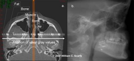
Figure 3. Ray Sum Images. An axial projection (a.) is used as the reference image. A section slice is identified (orange) which, in this case, corresponds to the mid-sagittal plane and the thickness of this increased to include both left and right sides of the volumetric dataset. As the thickness of the "slab" increases, adjacent voxels representing elements such as air, bone and soft tissues are added. The resultant image generated (b.) provides a simulated lateral cephalometric (Images generated using i-CAT CBCT; Danaher/Imaging Sciences International, Hatfield, PA)
2) 3D Volume Rendering. Volume rendering refers to techniques which allow the visualization of 3D data by selective display of voxels.
Techniques that integrate large volumes of adjacent voxels are classified as direct volume rendering (DVR) or indirect volume rendering (IVR). IVR is a complex process, requiring selection of the intensity or density of the grayscale level of the voxels to be displayed within an entire dataset (called "segmentation").This is technically demanding as it is necessary for the operator to provide either pre-set or manual inputs as to which voxels should be included. It is also computationally difficult, requiring specific software. However, the process provides a volumetric surface reconstruction with depth. (Figure 4)
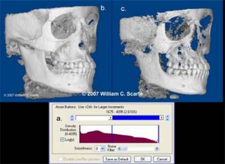
Figure 4. 3D Volumetric Surface Rendering. Manual segmentation is often accomplished using an adjustable scale determining the upper and lower limit and range of intensity values to include in the segmentation (lower screen). The visual result of changes in this scale is displayed in "real time" so that the effects of incremental changes can be visualized. Good segmentation provides an accurate representation of the osseous anatomy with minimal inclusion of noise or soft tissue (left image) whereas poor segmentation results in less noise but areas with less cortical thickness or lower intensity are under represented resulting in defects (right image). (Segmentation performed using Dolphin 3D, Chatsworth, CA)
DVR is a much more simple process. The most common DVR technique is maximum intensity projection (MIP). Each technique has advantages and disadvantages when used in clinical practice, and it is important that clinicians understand when and how each technique should be used. The purpose of the remaining discussion is to describe the maximum intensity projection technique and provide guidance on the application of this volume rendering method in cone beam CT based maxillofacial imaging
Maximum Intensity Projection (MIP)
Maximum intensity projection (MIP) was one of the first volume visualization techniques and probably is the most widely used methods in medical imaging because of the surprising simplicity and user-friendly algorithm. MIP is a 3D visualization technique that is achieved by evaluating each voxel value along an imaginary projection ray from the observer's eyes within a particular volume of interest and then representing only the highest value as the display value.6,7 Depending on the quality requirements of the resulting image, different mathematical strategies for finding the maximum value along a ray can be used.8-10 Voxel intensities below an arbitrary threshold are eliminated (Figure 5).
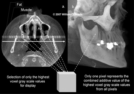
Figure 5. Maximum Intensity Projection Technique. This method of voxel vision produces an image by evaluating each voxel value along an imaginary projection ray from the observer's eyes within the dataset and then representing only the highest value as the display value. In this example, an axial projection (a.) is used as the reference image. A projection ray is identified (orange) throughout the entire volumetric dataset along which individual voxels are identified, each with varying grayscale intensity corresponding to various tissue densities such as fat, muscle, air and bone. The MIP algorithm selects only those values along the projection ray which have the highest values (corresponding usually to bone) and represents this as only one pixel on the resultant image (b.) (Images generated using i-CAT CBCT; Danaher/Imaging Sciences International, Hatfield, PA)
MIP algorithms determine the threshold for inclusion by considering the full range of intensities in the imaging volume, including quality signal and (interfering) noise. All information is rendered at the same level of intensity therefore, residual noise can become as conspicuous as anatomy. Some MIP programs provide options to optimize the performance of MIP rendering directed towards identifying noncontributing voxels and selectively eliminating them from the rendering process (Figure 6).
MIP algorithms determine the threshold for inclusion by considering the full range of intensities in the imaging volume, including quality signal and (interfering) noise. All information is rendered at the same level of intensity therefore, residual noise can become as conspicuous as anatomy. Some MIP programs provide options to optimize the performance of MIP rendering directed towards identifying noncontributing voxels and selectively eliminating them from the rendering process (Figure 6).
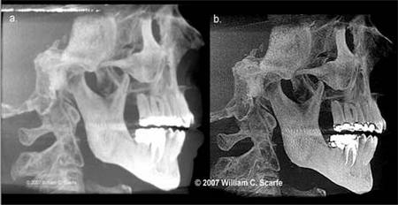
Figure 6. Stray Pixel Correction. High intensity grayscale artifacts, created due to scatter radiation or as a result of the cone beam effect can be represented as noise on MIP images. In this instance, the original full thickness MIP image (a.) demonstrates unwanted noise at the level of the amalgam restorations and at the upper edge whereas image (b.) has had a stray pixel correction applied. Note that while this reduces the effects mentioned, the resultant image is somewhat darker and grainier. (Images generated using iVISION, Danaher/Imaging Sciences International, Hatfield, PA)
The principal benefit of this method is to provide an operator-independent, "pseudo" 3D reconstruction representative of the volumetric dataset. In addition, because only data with the highest value are used, MIP images usually contain 10% or less of the original data and are therefore generated rapidly. MIP is particularly useful in representing the bony surface morphology of the maxillofacial region.
In addition, MIP is extremely useful for evaluating and locating high 'contrast', high attenuating substances. In medical imaging, this is particularly important to visualize contrast filled structures such as vessels. In maxillofacial imaging, it is often better than surface rendered 3D images to evaluate the location of third molars (Figure 7) or can be applied to evaluate the presence of a foreign body material or calcification in soft tissue structures. It is best used when the objects to be investigated are the 'brightest' objects in the image.
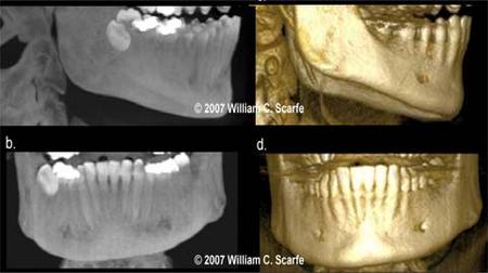
Figure 7. MIP vs. 3D Surface Rendering. Comparison of MIP (a. and b.) and 3D surface rendered (c. and d.) images generated from a sagittal (a. and c.) and coronal (b. and d.) projections. Unlike the surface renderings, which display the surface features of the volumetric dataset, MIP images inherently demonstrate all highly attenuating structures, irrespective of whether these are on the surface or not. This provides MIP images with an "opaque glass" feature, allowing features within the bone to be visualized. In this example, the location and depth of the mesio-angular impacted third molar in the mandibular right is more clearly demonstrated using sagittal and coronal MIPs than the 3D surface renderings. (3D Images generated using 3DVR Danaher/Imaging Sciences International, Hatfield, PA)
Despite their utility, MIPs present with one main limitation which the clinician must appreciate as the image is interpreted. An MIP image has a limited ability to represent anatomical spatial interrelations. This is because it does not contain shading information or visual clues for perception depth.
Therefore MIPs have a tendency to misrepresent positions because the projection technique doesn't take spatial location into account - only the maximal or (most attenuated) value is displayed. Therefore some structures may be obscured which may lead to sub-optimal interpretation of images. This concept is particularly important to comprehend the limitations of this technique when viewing full thickness MIP images in the orthogonal projections (Figure 8). In such situations, it is advisable to employ volume rendered 3D projection techniques in conjunction with MPR projections to assist in the interpretation process.
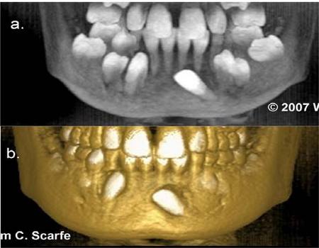
Figure 8. MIP Limitations in Spatial Relationships. MIP images have limitations in illustrating relative position and location because structures with higher value voxels lying behind a lower valued voxel appear to be in front of it. In this example of a patient with multiple mandibular impactions, the MIP image (a.) demonstrates the relative angulation of the unerupted and impacted mandibular left canine but provides no information on its relative bucco-lingual position. The 3D surface rendering (b.) however clearly demonstrates the buccal position of the crown. (3D Images generated using 3DVR Danaher/Imaging Sciences International, Hatfield, PA)
One technique to overcome this inherent limitation is to minimize the thickness and/or volume of the MIP image. This is referred to as Limited Volume MIP. Limiting the volume under consideration can improve pixel selection and enhance the accuracy of maximum intensity pixel projection. The ability to create an image based on regions of anatomy for inclusion or exclusion in the MIP is widely available and commonly employed. Isolating individual structures under evaluation, (e.g. bilateral structures of the maxilla) improves the accuracy of rendering and reduces overlap with adjacent structures (Figure 9).
One technique to overcome this inherent limitation is to minimize the thickness and/or volume of the MIP image. This is referred to as Limited Volume MIP. Limiting the volume under consideration can improve pixel selection and enhance the accuracy of maximum intensity pixel projection. The ability to create an image based on regions of anatomy for inclusion or exclusion in the MIP is widely available and commonly employed. Isolating individual structures under evaluation, (e.g. bilateral structures of the maxilla) improves the accuracy of rendering and reduces overlap with adjacent structures (Figure 9).
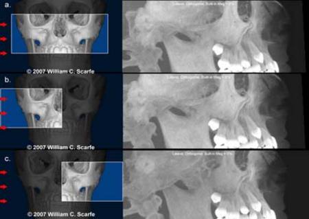
Figure 9. Limited volume MIP. One inherent limitation of MIP images is that bilateral structures are overlapped to form a "composite" image which may not represent the actual volume. In this example, a patient with bilateral, impacted and unerupted maxillary canines, the 3D surface rendering is unable to demonstrate the position of the teeth. Generation of a sagittal MIP using the entire volume of the maxilla (a.) provides a composite image representing both sides. Generation of a right (b.) and left (c.) limited volume MIP indicates remarkable symmetry in the position of the impacted canines and in the eruption sequence of the remaining unerupted teeth. (Images generated using Dolphin 3D, Chatsworth, CA)
Another approach, yet to be routinely available in maxillofacial imaging, is to animate the projection while viewing or to modulate the data values by their depth to achieve a kind of depth shading.11Overlapping, limited volume (OLIVE) MIP rendering can overcome many of the limitations of full-volume and regionally circumscribed MIP. These studies, also known as "sliding thin-slab MIPs"12 are essentially a hybrid between multi-planar reformation and MIP. To obtain this MIP, a thinslab MPR is selected from which an MIP image is reconstructed. This slab is moved through the volume, with the slab movement distance smaller than the slab thickness, and at each step an MIP is created. Applications include implant site and TMJ assessment (described later)
Applications of MIP Images in Maxillofacial Imaging
In medical imaging, MIP algorithms are used most often to depict volumetric vascular data sets acquired with both computed tomography12-15 and magnetic resonance.16, 17 However in maxillofacial CBCT imaging the use of MIP images have not been fully described. In our experience, MIP images have great utility in a number of specific clinical applications.
Impacted teeth
Successful surgical planning of impacted teeth depends on accurate localization, an understanding of orientation, depth and angulation and appreciation of proximity and relationship to other anatomic structures. MIP is of great value in the assessment of impacted teeth, providing the clinician with the ability to generate multiple 3D image projections at various angles with inherent image transparency (Figure 10).
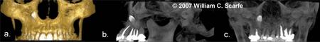
Figure 10. MIP in the Assessment of Impacted teeth. In this example, a patient presents with an impacted maxillary right canine. The 3D shaded surface volume rendering (a.) provides little information for surgical planning apart for indicating that the crown is erupting at the lateral border of the right lateral nasal fossa. Full thickness sagittal (b.) and coronal (c.) MIP images clearly demonstrate that the tooth is inverted, the root is straight and that the tooth is embedded vertically (3D image created with 3DVR, Danaher/Imaging Sciences International, Hatfield, PA).
Implant Imaging
For implant site assessment, the most common display format for CBCT imaging is based on a CT workstation programs such as Dentascan (GE Healthcare, Chalfont St. Giles, UK) and ToothPix (Cemax, Fremont, CA, USA), developed for conventional CT images more than 20 years ago.18, 19 These image display protocols are used to visualize the available alveolar bone and important anatomic structures.20
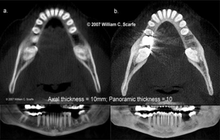
Figure 11. MIP in Implant Imaging. In this example, 10mm ray sum images (a.) are useful in that they provide an indication of the maximum available bucco-lingual width (axial view) and information of the orientation of the cross-sectional slices with respect to the occlusal and mandibular planes as well as the alveolar crest (panoramic view). 10mm OLIVE MIP images (b.) provide better visualization of the occlusal topography of the crowns of the teeth and alveolar crest (note the residual extraction defects) (axial view) and localize the position of the mental foramen in relation to the dentition (panoramic view).
Images usually include thin slice axial and panoramic oblique planar reference images as well as cross-sectional serial trans-planar images. While most information is obtained from the cross-sectional images, panoramic and axial views are often used to identify and locate important reference structures. In our experience, we often supplement the standard display formats with 10mm thick OLIVE MIP images in the axial view to provide better visualization of the occlusal topography of the crowns of the teeth and alveolar crest and in the panoramic view to localize the position of the mental foramen in relation to the dentition.
TMJ Evaluation
Narrow interval, overlapping sub-volume MIP slabs offer a valuable tomographic assessment augmenting evaluation of TMJ condylar orientation and shape (Figure 12). Limiting the volume in MIP reconstruction improves the integrity of MIP, limits overlap from adjacent bony structures and provides greater visualization of thinly corticated structures
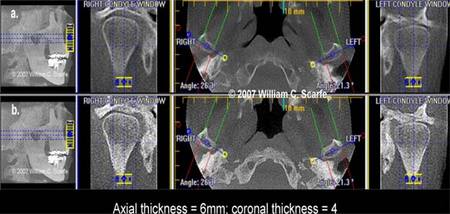
Figure 12. OLIVE MIP in TMJ Evaluation. In this example, the far left images provide a reference MIP sagittal image indicating localization of the axial slice to the level of the TMJ articulation. The para-coronal corrected images (labeled "right and left condyle window") in the 4mm MIP images (b.) more clearly demonstrate the integrity and relationship of the cortical bone of the TMJ condyles and shape of the glenoid fossa than the 4mm thick ray sum images (a.). In addition, the 6mm thick axial MIP images (b.) more clearly illustrate the long axis orientation of the condyles than the ray sum images (a.).(Images generated using iVISION, Danaher/Imaging Sciences International, Hatfield, PA)
Fractures
MIP images demonstrate disruption and discontinuity of osseous structures well. Heiland et al.21 first described an example of the use of MIP images for visualization of fractures of the maxillofacial region using a mandibular fracture. We have developed a simple protocol to demonstrate mandibular fractures in combination with other display modalities (Figure 13). The basis of the protocol is to represent limited volume MIPS in the region of interest in three planes. Initially bilateral linear oblique 10mm thick MPR images are created based on the axial image and MIP applied (Figure 13a). This provides lateral representations of the mandible (Figures 13b and c). Second, the location of the axial slice is positioned half way between the superior-inferior extent of the fracture and the thickness increased to include the full extent of the fracture and the MIP applied (Figure 13d). Finally, the location of the coronal slice is positioned half way between the anterior posterior extent of the fracture, increased to include the full extent of the fracture and the MIP applied (Figure 13e). This series of images provides adequate visualization of the extent, direction, and degree of displacement of most fractures.
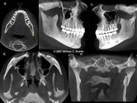
Figure 13. MIPs for Fractures. This MIP image sequence clearly demonstrates a simple slightly displaced fracture of the right parasymphyseal region. There is also a comminuted displaced left sub-condylar neck fracture. The condylar head fragment is displaced laterally, inferiorly and somewhat anteriorly and has translated towards the lateral rim of the glenoid fossa. The inferior mandibular ramus segment has rotated superiorly and slightly posteriorly. Between the two segments there is a triangular-shaped slither of bone obliquely positioned between the ramal and condylar segments.
Calcifications
Calcifications within soft tissue have higher voxel grayscale intensity values than the neighboring voxels and therefore appear as bright spots on MIP images. Thus MIP provides valuable information on the distribution and location of soft tissue vascular calcifications. This is particularly valuable in the identification and demonstration of tonsilloliths, salivary gland stones, calcified lymph nodes and carotid artery calcifications (Figure 14).
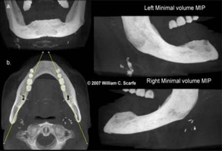
Figure 14. MIPs for Calcifications. This patient presented for implant site assessment of the mandible. The medical history revealed a previous history of carotid artery endarterectomy on the patient's right side. Frontal (a.) and axial (b.) full thickness MIP images demonstrated highly attenuating material bilaterally, immediately inferior to the angle of the mandible. Minimal volume (40mm thickness) bilateral planar linear MPR reconstructions identify the artery clips used in the right endarterectomy however also reveal substantial calcifications consistent with carotid artery calcifications at the level of the bifurcation on the left.
Craniofacial Anomalies
Imaging plays an important role in the diagnosis of craniosynostosis. Patients with suspected craniosynostosis are usually studied with 2D and 3D CT and/or plain radiography. However there are numerous limitations in the use of CT in examining these patients. 2D axial CT images may not show suture patency well if the plane of sectioning is running parallel to the suture. In addition, 3D shaded surface display may blend an open suture with the adjacent calvarial bone, providing an overestimation of the condition or may not display peri-sutural sclerosis well, which may be seen in early sutural closure. Medina22 first described the application of MIP images in conventional CT images for the assessment of craniofacial anomalies. Araki et al. demonstrated the application of this technique for cleft palate and lip applications.23Based on this work, we have developed a protocol (Figure 15) which we have found particularly useful in providing a convenient standardized presentation format for full assessment of all the sutures and calvarial bones.
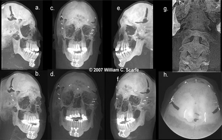
Figure 15. MIPs for Craniofacial Anomalies. MIP images provide a convenient method to visualize the complex relationships of the maxillofacial bones. A standard eight projection series comprising 100mm thick right (a.) and left (e.) sagittals, right (b.) and left (f.) 450 frontal obliques, frontal (c.) and 400 frontal (d.) obliques, occipital (h.) and cervical images (g.) provides a full assessment of the deficiencies in sutural closure and bone formation associated with craniosynostosis.
Cervical Spine
The cervical spine is a structural feature often included in CBCT scans of the maxillofacial region, particularly with larger field of view protocols. It is not routinely imaged. However it is important to recognize that congenital anomalies of the cervical spine have been associated with osteogenesis imperfecta and with various craniofacial anomalies including Crouzon24 and Pfeiffer's25 syndromes, hemifacial microsomia26 and, in particular, Goldenhar's Syndrome.27
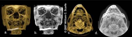
Figure 16. MIPs for Post Operative Assessment. Comparison of frontal (a.) and SMV (d.) 3D surface renderings with frontal (b.) and inferior (c.) MIP images for a patient who was reconstructed with tibia graft material stabilized with surgical plates after pathologic fracture associated with mandibular atrophy.
Cervical anomalies present as a failure of formation, failure of segmentation or combinations of both failure of formation and formation. Initial evaluations of the cervical spine with conventional plain film radiography includes anteroposterior, an open-mouth odontoid and lateral neutral, flexion, and extension projections.28 MIP can be readily applied at these modifed projections to demonstrate the extent and nature of cervical anomaly (Figure 17).
Cervical anomalies present as a failure of formation, failure of segmentation or combinations of both failure of formation and formation. Initial evaluations of the cervical spine with conventional plain film radiography includes anteroposterior, an open-mouth odontoid and lateral neutral, flexion, and extension projections.28 MIP can be readily applied at these modifed projections to demonstrate the extent and nature of cervical anomaly (Figure 17).
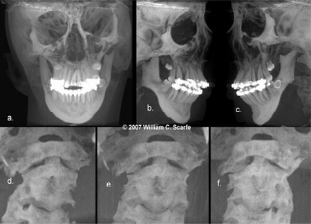
Figure 17. MIPs for Cervical Spine Assessment. Standard full field of view MIP images comprising coronal (a.) and right (b.) and left (c.) corrected projections demonstrate the maxillofacial facial features associated with this patient with Goldenhar's Syndrome. In addition, limited volume (50mm thickness) 450 oblique (d.), coronal (e.) and left 450 oblique (f.) MIP projections clearly demonstrate compensatory cervical spine scoliosis with marked deviation to the right and anteriorly with fusion of the anterior vertebral bodies of C2 and C3.
Orthodontic Analysis
Because MIP images clearly demonstrate the surface features of the maxillofacial complex, they are particularly useful in establishing the location of topographic landmarks. Orthodontic tracings using a combination of ray sum and MIP images are particularly useful. The ray sum image provides a simulated lateral cephalometric view of the maxillofacial region and, being transparent, provides identification of mid-sagittal features such as Sella and posterior nasal spine (PNS) (Figure 18a). However ray sum images suffer the same limitations as conventional images in that they provide limited identification of surface features. In comparison, MIP images more clearly allow identification of landmarks associated with curved surfaces (e.g. Orbitale, zygomatic arch), sutures (Nasion), orifices (e.g. Porion) and thinner structures (e.g. Point A and anterior nasal spine) (Figure 18b). The use of supplemental images can potentially increase the reliability and accuracy of measurements obtained from cephalometric analysis. One orthodontic software package (Dolphin Imaging V.10.5, Chatsworth CA) allows for import and analysis of CBCT DICOM data (Dolphin 3D, Chatsworth CA) and provides for standard planar orthodontic projections that can be visualized in multiple display modes, including MIP, facilitating orthodontic analysis and potentially reducing errors associated with landmark identification.
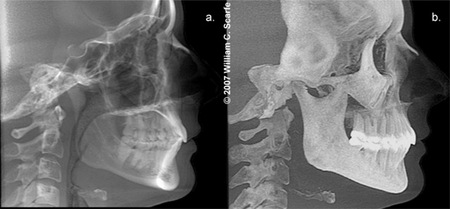
Figure 18. MIPs for Cephalometric Orthodontic Analysis.Comparison of simulated lateral cephalometric ray sum (a.) and MIP (b.) images produced using Dolphin 3D (Dolphin Imaging v.10.5, Chatsworth, CA). When imported into Dolphin cephalometric analysis program, these images plus additional display modes (enhanced ray sum, embossed and tracing mode) can be alternately superimposed to compare the location of specific landmarks. Note the clarity with which notoriously difficult topographic landmarks on conventional ray sum images (e.g. ANS, porion, orbitale, nasion) are easily identified on the MIP images.
Conclusion
The MIP is a simple, easily applied 3D visualization tool that can be used to display CBCT volumetric datasets. While this technique can assist the clinician in providing some degree of "Voxel Vision" in numerous clinical situations, it should always be used as an adjunct, not as a replacement, to thorough and systematic evaluation of the constructed CBCT images.
REFERENCES
- Cohnen M, Kemper J, Mobes O, Pawelzik J, Modder U. Radiation dose in dental radiology. Eur Radiol 2002;12:634-7.
- Schulze D, Heiland M, Thurmann H, Adam G. Radiation exposure during midfacial imaging using 4- and 16-slice computed tomography, cone beam computed tomography systems and conventional radiography. Dentomaxillofac Radiol 2004;33:83-6.
- Heiland M, Schulze D, Rother U, Schmelzle R. Postoperative imaging of zygomaticomaxillary complex fractures using digital volume tomography. J Oral Maxillofac Surg 2004;62:1387-91.
- Mah JK, Danforth RA, Bumann A, Hatcher D. Radiation absorbed in maxillofacial imaging with a new dental computed tomography device. Oral Surg Oral Med Oral Pathol Oral Radiol Endod 2003;96:508-13.
- Ludlow JB, Davies-Ludlow LE, Brooks SL. Dosimetry of two extraoral direct digital imaging devices: NewTom cone beam CT and Orthophos Plus DS panoramic unit. Dentomaxillofac Radiol 2003;32:229-34.
- Cody DD. AAPM/RSNA physics tutorial for residents: topics in CT. Image processing in CT. Radiographics 2002;22:1255-68.
- Calhoun PS, Kuszyk BS, Heath DG, Carley JC, Fishman EK. Three-dimensional volume rendering of spiral CT data: theory and method. Radiographics. 1999;19:745-64.
- Sakas G, Grimm M, Savopoulos A. Optimized maximum intensity projection. Proceedings of 5th EUROGRAPHICS Workshop on Rendering Techniques, Dublin, Ireland 1995;pp.55-63.
- Zuiderveld KJ, Koning AHJ, Viergever MA. Techniques for speeding up high-quality perspective maximum intensity projection. Pattern Recognition Letters 1994;15:507-517
- Cai W, Sakas G. Maximum intensity projection using splatting in sheared object space. Proceedings EUROGRAPHICS '98 1998;pp.C113-C124,.
- Heidrich W, McCool M, Stevens J. Interactive maximum projection volume rendering. IEEE Proceedings Visualization '95 1995;pp.11-18.
- Napel S, Rubin GD, Jeffrey RB, Jr. STS-MIP: a new reconstruction technique for CT of the chest. J Comput Assist Tomogr 1993;17:832-838.
- Napel S, Marks MP, Rubin GD, et al. CT angiography with spiral CT and maximum intensity projection. Radiology 1992;185:607-610.
- van Ooijen PM, Ho KY, Dorgelo J, Oudkerk M. Coronary artery imaging with multidetector CT: visualization issues. Radiographics 2003;23:e16.
- Prokop M, Shin HO, Schanz A, Schaefer-Prokop CM. Use of maximum intensity projections in CT angiography: a basic review. Radiographics 1997;17:433-51.
- Laub GA, Kaiser WA. MR angiography with gradient motion refocusing. J Comput Assist Tomogr 1988;12:377-382.
- Schreiner S, Paschal CB, Galloway RL. Comparison of projection algorithms used for the construction of maximum intensity projection images. J Comput Assist Tomogr 1996;20:56-67.
- Abrahams JJ. Anatomy of the jaw revisited with a dental CT software program. AJNR Am J Neuroradiol 1993;14:979-90.
- Casselman JW, Deryckere F, Hermans R, Declercq C, Neyt L, Pattyn G, Meeus L, Vandevoorde P, Steyaert L, Devos V. Denta Scan: CT software program used in the anatomic evaluation of the mandible and maxilla in the perspective of endosseous implant surgery. Rofo 1991;155:4-10.
- Dentascan in oral imaging.Au-Yeung KM, Ahuja AT, Ching AS, Metreweli C. Dentascan in oral imaging. Clin Radiol 2001;56:700-13.
- Heiland M, Schmelzle R, Hebecker A, D Schulze D. 3Intraoperative 3D imaging of the facial skeleton using the SIREMOBIL IsoC3D. Dentomaxillofac Radiol 2004;33:130-2.
- Medina LS. Three-dimensional CT maximum intensity projections of the calvaria: a new approach for diagnosis of craniosynostosis and fractures. AJNR Am J Neuroradiol 2000;21:1951-4.
- Araki K, Maki K, Seki K, Sakamaki K, Harata Y, Sakaino R, Okano T, Seo K. Characteristics of a newly developed dentomaxillofacial X-ray cone beam CT scanner (CB MercuRayTM): system configuration and physical properties. Dentomaxillofac Radiol 2004;33:51-9.
- Anderson PJ, Hall CE, Evans RD, Hayward RD, Harkness WJ, Jones BM. Cervical spine anomalies in Crouzon syndrome. Spine 1997;22:402-5.
- Anderson PJ, Hall CE, Evans RD, Hayward RD, Harkness WJ, Jones BM. Cervical spine anomalies in Pfeiffer's syndrome. J Craniofac Surg 1997b;7:275-9.
- Figueroa AA, Friede H. Craniovertebral malformations in hemifacial microsomia. J Craniofac Genet Dev Biol 1985;1(suppl):167-78.
- Gosain AK, McCarthy JG, Pinto RS. Cervicovertebral anomalies and basilar impression in Goldenhar syndrome. Plast Reconstr Surg 1994;93:498-506.
- Brinker MR, Weeden SH, Whitecloud TS 3rd. Congenital anomalies of the cervical spine. In: Frymoyer JW, editor. The adult spine: principles and practice. Philadelphia:Lippincott-Raven 1997;pp.1205-22.